最適輸送解析ダッシュボード
Optimal Transport Analysis Dashboard
A状態→B状態→C状態 分岐パターン解析
State A → State B → State C Branching Pattern Analysis
📈 最適輸送問題の概要
📐 最適輸送問題の基本的な考え方
ある確率分布に従う質量(あるいは確率)を、別の確率分布に移動させるために必要なコストを最小化するような輸送方法を求める問題です。
🕰️ 最適輸送問題の歴史
1942年
カントロヴィッチ (Kantorovich): ソ連の数学者・経済学者レオニード・カントロヴィッチがモンジュの古典的輸送問題を線形計画法の枠組みで緩和・一般化し、「輸送計画(transport plan)」の概念を導入。
1975年
🏆 ノーベル経済学賞: カントロヴィッチは「資源配分理論への貢献」によりノーベル経済学賞を受賞しました。
1990年代
計算手法の進歩: 計算手法の進歩により、特にコンピュータビジョン領域で「Earth Mover's Distance(EMD)」として実装され、画像検索やテクスチャ解析への応用が始まりました。
2010年代以降
🚀 現代応用: 深層学習分野ではWasserstein GAN(WGAN, 2017)が提案されて生成モデルの安定化に貢献。生物学分野では単一細胞データの発生軌跡推定(Waddington-OT, 2019)など最先端応用が急速に拡大。
🧮 最適輸送問題の数学的な基礎 ▼
🎯 最適輸送解析の核心的なポイント
「離散的なスナップショットデータから連続的な変化プロセスを推定できる」
実際には時系列ではないデータ(異なる状態の独立したサンプル)に対して、連続性を仮定することで、状態間の滑らかな遷移経路を数学的に復元できます。これにより、観測されていない「中間プロセス」を理論的に推定し、変化のメカニズムを解明できるのが最適輸送解析の革新的な価値です。
⚠️ 仮定と限界 ▼
🎬 状態遷移パターン
🎬 動的遷移アニメーション
各データポイントが早期状態から中期状態、そして2つの後期状態への最適経路に沿って遷移する様子を示すアニメーション
🔧 アニメーション技術仕様
- 解像度: 1920×1440ピクセル(高解像度)
- フレーム数: 各状態15フレーム(滑らかな遷移)
- 色分け: A(青) → B(緑) → C1(赤)/C2(オレンジ)
- 透明度: 視認性を保つためのアルファ値調整
- 軌跡表示: 各データポイントの個別移動経路
- 統一軸範囲: 密度分布版と同じXY軸範囲で一貫した比較を可能に
📊 密度分布付きアニメーション
状態の変化パターンを密度分布と等高線で可視化。データポイントの集中度と分散パターンが明確に表示されます
🎨 密度可視化の特徴
- 密度等高線: 各状態の分布密度を等高線で表示
- 固定密度閾値: アニメーション全体で一貫した密度レベル(0.1, 0.3, 0.5, 0.7, 0.9)を使用
- コンパクトな密度分布: 小さく調整された密度分布でデータポイントの集中度を精密に表現
- 統一軸範囲: 基本版と同じXY軸範囲(15%拡張)で直接比較を可能に
- シンプルデザイン: 背景色を排除し、等高線のみで密度パターンを表現
- 統計的解釈: 分布の形状変化から遷移パターンを定量化
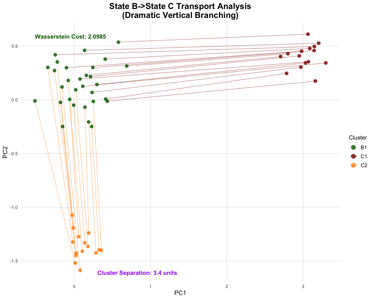
- クラスター分析: 状態Cでの2つの分岐パターンを明確に可視化
🎯 状態遷移の可視化
📊 状態遷移の模式図
A
初期状態
B
中間状態
C1
最終状態1
C2
最終状態2
🔍 遷移パターンの特徴
- A → B: 単一方向への集約的遷移(30データポイント全てが同じ中間状態へ)
- B → C1/C2: 分岐的遷移(中間状態から2つの異なる最終状態への分散)
- 色分け: A(青) → B(緑) → C1(赤)/C2(オレンジ)で状態を明確に区別
- 分岐比率: C1とC2への分岐は約50:50の比率で発生
📊 静的図表 (PNG)
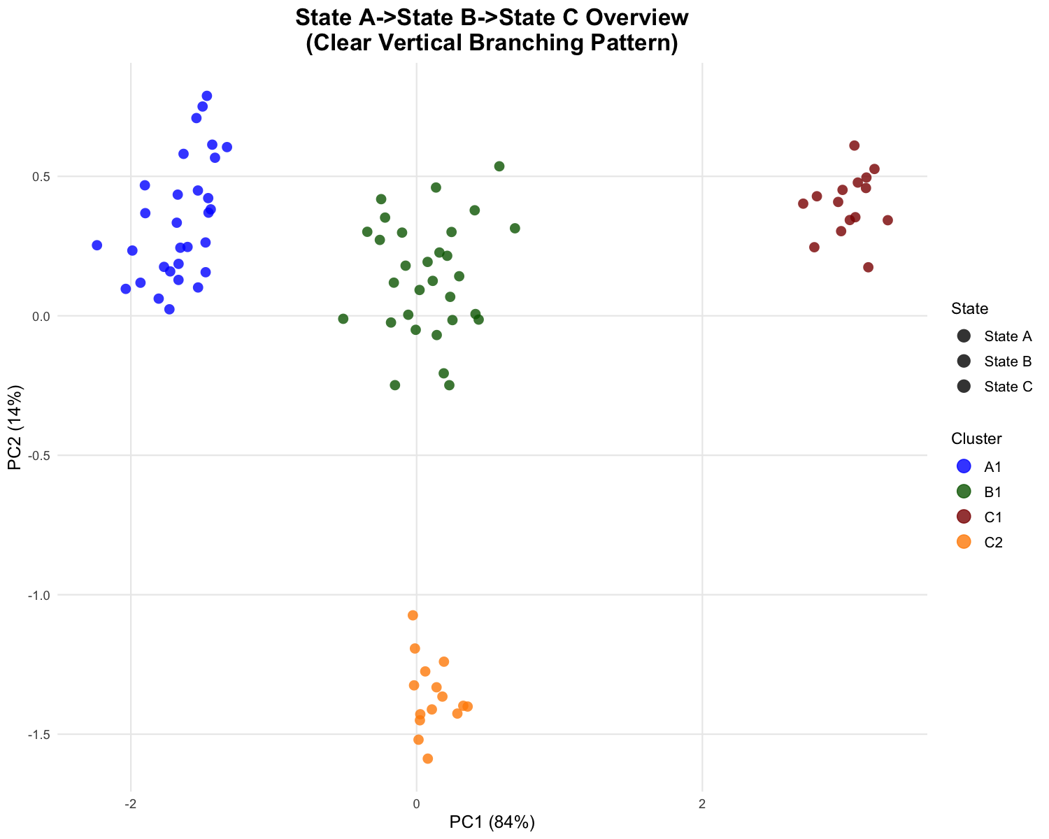
State A→State B→State Cの全体的な分岐パターンを示す静的図表(Cluster: A1, B1, C1, C2)
➡️ A→B輸送可視化
📊 静的図表 (PNG)
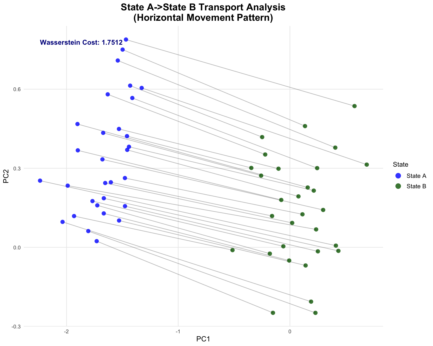
State AからState Bへの最適輸送パターンと矢印による移動経路の可視化
💻 A→B輸送の実行コード (R)
# A→B輸送解析のRコード (mvp_simple.Rより)

# PNG 2: A→B Transport using ggplot2
cat("Creating transport_ab.png with ggplot2...\n")

# Prepare A→B data
ab_data <- data.frame(
  PC1 = c(pca_A$data[,1], pca_B$data[,1]),
  PC2 = c(pca_A$data[,2], pca_B$data[,2]),
  State = factor(c(rep("State A", nrow(pca_A$data)),
                   rep("State B", nrow(pca_B$data))),
                 levels = c("State A", "State B"))
)

# Prepare ALL transport arrows (not sampled)
ab_arrows <- data.frame()
if(nrow(transport_AB$plan) > 0) {
  for (i in 1:nrow(transport_AB$plan)) {
    if (transport_AB$plan[i, 3] > 1e-6) {
      ab_arrows <- rbind(ab_arrows, data.frame(
        x = pca_A$data[transport_AB$plan[i, 1], 1],
        y = pca_A$data[transport_AB$plan[i, 1], 2],
        xend = pca_B$data[transport_AB$plan[i, 2], 1],
        yend = pca_B$data[transport_AB$plan[i, 2], 2],
        weight = transport_AB$plan[i, 3]
      ))
    }
  }
}

p2 <- ggplot(ab_data, aes(x = PC1, y = PC2)) +
  geom_segment(data = ab_arrows, aes(x = x, y = y, xend = xend, yend = yend),
               arrow = arrow(length = unit(0.15, "cm")),
               color = "gray40", linewidth = 0.5, alpha = 0.4) +
  geom_point(aes(color = State), size = 3, shape = 16, alpha = 0.8) +
  scale_color_manual(values = c("State A" = "blue", "State B" = "darkgreen")) +
  labs(title = "State A->State B Transport Analysis\n(Horizontal Movement Pattern)",
       x = "PC1", y = "PC2") +
  annotate("text", x = min(ab_data$PC1), y = max(ab_data$PC2),
           label = paste("Wasserstein Cost:", round(transport_AB$cost, 4)),
           hjust = 0, vjust = 1, size = 4, fontface = "bold", color = "darkblue") +
  theme_minimal() +
  theme(
    plot.title = element_text(size = 16, hjust = 0.5, face = "bold"),
    axis.title = element_text(size = 12),
    legend.position = "right",
    legend.title = element_text(size = 11),
    legend.text = element_text(size = 10),
    panel.grid.minor = element_blank()
  ) +
  guides(color = guide_legend(title = "State", override.aes = list(size = 4)))

ggsave("transport_ab.png", plot = p2, width = 10, height = 8, dpi = 150, bg = "white")
cat("✅ Generated: transport_ab.png with ggplot2 (all arrows displayed)\n")